This dataset summarises benthic surveys of seagrass for Dugong and Turtle habitats in the North-West Torres Strait for November 2015 and January 2016. The Site data describes seagrass at 853 sites; while the Meadow data describes seagrass at 34 individual meadows. The data includes information on seagrass species, biomass, diversity, and BMI and algae percent cover. The dataset is available as shapefiles, GIS layer packages, and/or a CSV file. Methods: The sampling methods used to study, describe and monitor seagrass meadows were developed by the TropWATER Seagrass Group and tailored to the location and habitat surveyed; these are described in detail in the relevant publications (https://research.jcu.edu.au/tropwater). 1. Location - Latitude and longitude was recorded by GPS at each site. Depth was recorded when sampling by boat and converted to depth below mean sea level (dbMSL) in metres. 2 Seagrass metrics - Above-ground biomass was determined using a “visual estimates of biomass” technique (Mellors, 1991) using trained observers. A linear regression was calculated for the relationship between the observer ranks and the harvested values. This regression was used to calculate above-ground biomass for all estimated ranks made from the survey sites. Biomass ranks were then converted into above-ground biomass estimates in grams dry weight per square metre (gdw m-2). Observers ranked seagrass biomass, and the percent contribution of each species to that biomass, using video transects, grabs, free divers, and helicopter: * Video transect: Commonly used for subtidal meadows sampled from larger boats. At each transect site an underwater CCTV camera system was lowered from the vessel to the bottom. For each transect the camera was towed at drift speed (less than one knot) for approximately 100m. Footage was observed on a TV monitor and digitally recorded. The video was paused at ten random time frames and an observer ranked seagrass biomass and species composition. On completion of the video analysis, the video observer ranked five additional quadrats that had been previously videoed for calibration. These quadrats were videoed in front of a stationary camera, then harvested, dried and weighed. * Helicopter: Commonly used for intertidal surveys. At each site seagrass above-ground biomass and species composition were estimated from three 0.25 m2 quadrats placed randomly within a 10m2 circular area. Seagrass percent cover and sediment type were recorded at each site. The “visual estimates of biomass” technique when applied to helicopter surveys (and free diving/camera drops – see below) involves ranking while referring to a series of quadrat photographs of similar seagrass habitats for which the above-ground biomass has previously been measured. Three separate biomass scales were used: low-biomass, high-biomass, and Enhalus-biomass. The relative proportion (percentage) of the above-ground biomass of each seagrass species within each survey quadrat was also recorded. Field biomass ranks were converted into above-ground biomass estimates in grams dry weight per square metre (gdw m-2). At the completion of sampling each observer ranked a series of calibration quadrats as per video transect surveys. * Camera drop/free diving: Commonly used for shallow subtidal meadows sampled from a small boat. Sampling follows the same protocol as helicopter surveys but the three quadrats were either assessed by a free diver with quadrat, or by an underwater CCTV camera system camera attached to a frame. Video footage was observed on a TV monitor and seagrass ranked in real time, with the camera frame serving as a quadrat. * van Veen grab: Commonly used for shallow subtidal meadows sampled from a small boat in conjunction with camera drops, or to record seagrass presence/absence where visibility was too poor for camera drops. A sample of seagrass was collected using a van Veen grab (grab area 0.0625 m2) to identify species present at each site. Species identified from the grab sample were used to inform species composition assessments made from the video drops (Kuo et al., 1989). 3 Benthic macro-invertebrates - A visual estimate of benthic macro-invertebrate (BMI) percent cover was recorded at each shallow subtidal and intertidal site according to four broad taxonomic groups: * Hard corals – All scleractinian corals including massive, branching, tabular, digitate and mushroom. * Soft corals – All alcyonarian corals, i.e. corals lacking a hard limestone skeleton. * Sponges * Other BMI – Any other BMI identified, e.g. hydroids, ascidians, barnacles, oysters, molluscs. Other BMI are listed in the “comments” column of the GIS site layer. 4 Algae - A visual estimate of algae percent cover was recorded at each shallow subtidal and intertidal site. When present, algae were categorised into five functional groups and the percent contribution of each functional group was estimated: * Erect macrophytes – Macrophytic algae with an erect growth form and high level of cellular differentiation, e.g. Sargassum, Caulerpa and Galaxaura species. * Erect calcareous – Algae with erect growth form and high level of cellular differentiation containing calcified segments, e.g. Halimeda species. * Filamentous – Thin, thread-like algae with little cellular differentiation. * Encrusting – Algae that grows in sheet-like form attached to the substrate or benthos, e.g. coralline algae. * Turf mat – Algae that forms a dense mat on the substrate. Format: This dataset consists of two (2) GIS layers: a Site layer and a Meadow layer. 1. Site layer This layer contains data collected at 853 individual survey sites mapped in 2015-2016, and includes: * Temporal details - survey date and time. * Spatial details – latitude/longitude, dbMSL, sediment type, NRM region, site depth (depth below mean sea level, m). * Habitat information – seagrass presence absence, dominant seagrass species, presence/absence of individual species, seagrass above-ground biomass (for each species), Shannon-Weaver seagrass diversity values, dugong feeding trail presence/absence (intertidal sites only), and percent cover for seagrass, algae groups and benthic macro-invertebrates. * Sampling methods, any relevant comments, and data custodian. This layer is presented as five (5) alternate layer packages based on symbology from specific columns: * Seagrass presence/absence (Torres Strait seagrass present absent NESP 2015.lpk) * Seagrass species composition (Torres Strait seagrass species composition NESP 2015.lpk) * Dugong feeding trail presence absence (Torres Strait dugong feeding trail presence absence NESP 2015.lpk) (Note: this layer only includes site information for intertidal helicopter surveys) * Algae cover (Torres Strait algae cover NESP 2015.lpk) * Benthic macro-invertebrate cover (Torres Strait benthic macro-invertebrate cover NESP 2015.lpk) 2. Meadow layer Seagrass presence/absence site data was used to construct the polygon (meadow) layer. The meadow layer provides summary information for all sites within the meadow, and includes: * Spatial details – depth range of sites and meadow location. * Habitat information – seagrass species present, meadow community type and density, mean meadow biomass + standard error (s.e.), meadow area + reliability estimate (R) and number of sites within the meadow. * Sampling methods and any relevant comments. This layer is presented as three (3) alternate layer packages, including interpolation layers which were created using site data and meadow boundaries to describe spatial variation in biomass, species diversity and depth gradients. The layers are: * "Torres Strait meadow community type NESP 2015.lpk" - Includes 34 individual seagrass meadows mapped in 2015-2016 with information including individual meadow ID, meadow location (intertidal/shallow subtidal/subtidal), meadow density based on mean biomass, meadow area, dominant seagrass species, seagrass species present, survey dates, survey method, and data custodian. ESRI and Landsat satellite image basemaps were used as background source data to check meadow and site boundaries, and re-map where required. * "Torres Strait biomass (g dw m-2) interpolation NESP 2015.lpk" - An inverse distance weighted interpolation (IDW) was applied to seagrass site data to describe spatial variation in biomass across each meadow and throughout the north-west Torres Strait region. * "Torres Strait Shannon Weaver diversity interpolation NESP 2015.lpk" - An inverse distance weighted interpolation (IDW) was applied to seagrass site data to describe spatial variation in seagrass species diversity across each meadow and throughout the north-west Torres Strait region. The Shannon-Weaver index is a mathematical measure of species diversity that uses species richness (the number of species present, where a score of 0 = one species present) and the relative abundance of different species (Spellerberg et al., 2003). Data Dictionary: * Meadow location was classed according to whether meadows were intertidal (all sites surveyed by helicopter), shallow subtidal (generally an extension of an intertidal meadow into shallow waters <5m deep), or subtidal (no intertidal sites adjoining the meadow). * Seagrass community types were determined according to species composition within a meadow. Species composition was based on the percent each species’ biomass contributed to mean meadow biomass. A standard nomenclature system was used to categorize each meadow (see Table 1 "Nomenclature for seagrass community types" in final report). This nomenclature also included a measure of meadow density categories (light, moderate, dense) determined by mean biomass of the dominant species within the meadow (see Table 2 "Density categories and mean above-ground biomass ranges for each species used in determining seagrass community density" in final report). * Mapping precision estimates (in metres) were based on the mapping method used for that meadow (Table 3 "Mapping precision and methods for seagrass meadows" in final report). Mapping precision estimates ranged from 1-10m for intertidal seagrass meadows to >100m for patchy subtidal meadows. Subtidal meadow mapping precision estimates were based on the distance between sites with and without seagrass. The mapping precision estimate was used to calculate an error buffer around each meadow; the area of this buffer is expressed as a meadow reliability estimate (R) in hectares. Further information can be found in this publication: Carter, A. B. and Rasheed, M. A. (2016) Assessment of Key Dugong and Turtle Seagrass Resources in North-west Torres Strait. Report to the National Environmental Science Programme and Torres Strait Regional Authority. Reef and Rainforest Research Centre Limited, Cairns (40 pp). References: Kuo, J., & McComb, A. J. (1989). Seagrass taxonomy, structure and development. In A. W. D. Larkum, A. J. McComb, & S. A. Shepherd (Eds.), Biology of seagrasses: a treatise on the biology of seagrasses with special reference to the Australian Region (pp. 6-73). New York: Elsevier. Mellors, J. E. (1991). An evaluation of a rapid visual technique for estimating seagrass biomass. Aquatic Botany, 42(1), 67-73. Spellerberg, I. F., & Fedor, P. J. (2003). A tribute to Claude Shannon (1916–2001) and a plea for more rigorous use of species richness, species diversity and the ‘Shannon–Wiener’ Index. Global Ecology and Biogeography, 12(3), 177-179. Data Location: This dataset is saved in the eAtlas enduring data repository at: data\NESP1\3.5_North-West-TS_Seagrass

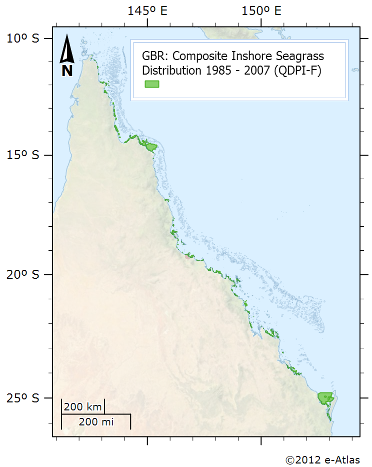
This dataset is shows the distribution of inshore seagrass along the eastern Queensland coastline. It is a composite of 38 surveys conducted from 1984 to 2007. Coastal seagrasses in waters shallower than -15 metres were mapped by dive surveys, under water cameras and inter-tidal aerial surveys. The data includes location information on the spatial extent of seagrass habitats mapped in 38 surveys between 1984 – 2007. The data does not include species information. Seagrass surveys were conducted at various times and at different precisions but the composite layer is the best depiction of seagrass for the GBRWHA and Hervey Bay presently available for planning purposes. Seagrass distribution can change seasonally and between years, and users should ensure that they make appropriate enquires to determine whether new or more appropriate information is available. Notes: This dataset is somewhat deprecated by a more recent compilation of seagrass data in 2015 that is openly available. See the related data link. Data Location: This dataset is filed in the eAtlas enduring data repository at: data\custodian\2006-2010-MTSRF\GBR_MTSRF-1-1-3_QDPI-F_Coles-R_Composite-seagrass-1984-2007

This dataset is consists of modelled habitat suitability of coastal seagrass distribution in the wet and dry seasons along the Great Barrier Reef World Heritage Area coastline. A Bayesian belief network was used to quantify the relationship (dependencies) between seagrass and eight environmental drivers: relative wave exposure, bathymetry, spatial extent of flood plumes, season, substrate, region, tidal range and sea surface temperature. We found that at the scale of the entire GBRWHA, the main drivers of inshore seagrass presence are tidal range and relative exposure. The outputs of our analysis included a probabilistic GIS-surface of inshore seagrass presence and distribution for both the wet and dry seasons, and across four regions at the scale of 2km*2km planning units. The model can be used by managers in the GBRWHA to delineate seagrass ecological units, and assist them in marine planning at broad spatial scales. For more information about methods see: Grech, A. and Coles, R.J. 2010, An ecosystem-scale predictive model of coastal seagrass distribution, Aquatic Conservation: Marine and Freshwater Ecosystems 20: 437-444 Data Location: This dataset is filed in the eAtlas enduring data repository at: data\MTSRF\QLD_MTSRF-1-1-3_JCU_Grech-A_Seagrass-coastal-model-2007

Pattern of seagrass distribution in the Great Barrier Reef World Heritage Area Seagrasses in waters deeper than 15m in the Great Barrier Reef World Heritage Area adjacent to the Queensland coast were surveyed using a camera and dredge towed for 4-6 minutes at 1,429 sites spanning from 10ºS to 25ºS and from inshore out to the reef edge up to 120nm from the coast. At each site seagrass presence, species and biomass were recorded together with depth, sediment, sechii, algae and epibenthos, and proximity to reefs. Seagrasses in this region extend down to 60 m water depths and are difficult to map other than by generating distributions from point source data. Statistical modelling of the seagrass distribution suggests 40,000 km^2 of the bottom has a probability of some seagrass being present. There is strong spatial variability driven in part by the constraint of the Great Barrier Reef’s long, thin shape and physical processes associated with the land and ocean. We map the four main species, Halophila ovalis, H. spinulosa, H. decipiens, and H. tricostata. Distributions of H. ovalis and H. spinulosa show strong depth and sediment effects, whereas H. decipiens, and H. tricostata are only weakly correlated with environmental variables but show strong spatial patterns. Distributions of all species are correlated most closely with depth and the proportion of medium sized sediment. As part of the Reef Atlas project (now the eAtlas) the seagrass observations were interpolated over the whole GBR by Glenn De'ath using Generalized Additive Models with a Quasibinomial fit. This produced a gridded version of the dataset and is available as a KML and ASCII grid file. Data Units: Probability of occurrence (0 to 1).

This dataset shows the effects of imazapic (detected in the Great Barrier Reef catchments) on the growth rate (from cell density data) on the cyanobacteria Microcystis aeruginosa over a 72 hour exposure period during laboratory experiments conducted in 2019. The aims of this project were to develop and apply standard ecotoxicology protocols to determine the effects of Photosystem II (PSII) and alternative herbicides on the growth of the cyanobacteria Microcystis aeruginosa. Growth bioassays were performed over 3-day exposures using imazapic which has been detected in the Great Barrier Reef catchment area (O’Brien et al. 2016). This toxicity data will enable improved assessment of the risks posed by the herbicide imazapic to cyanobacteria for both regulatory purposes and for comparison with other taxa. Methods: The cyanobacteria Microcystis aeruginosa (Kutzing) Kutzing 1846 (Cyanophyceae) (CS338/01) was purchased from the Australian National Algae Supply Service, Hobart (CSIRO). Cultures of M. aeruginosa were established in MLA medium (Bolch and Blackburn 1996). Cultures were maintained in sterile 250 mL Erlenmeyer flasks as batch cultures in exponential growth phase with weekly transfers of 1 - 3 mL of a 7 day-old M. aeruginosa suspension to 100 mL MLA medium under sterile conditions. Clean culture solutions were maintained at 26 ± 2°C, and under a 12:12 h light:dark cycle (91 ± 12 µmol photons m–2 s–1). Imazapic stock solution was prepared using PESTANAL (Sigma-Aldrich) analytical grade (HPLC greater than or equal to 98%) imazapic (CAS 104098-48-8). The selection of imazapic was based on application rates and detection in coastal waters of the GBR (Grant et al. 2017, O’Brien et al. 2016). Imazapic stock solution was prepared in 1 L volumetric flasks using milli-Q water. Imazapic was dissolved using analytical grade methanol (final concentration < 0.01% (v/v) in exposures). Cultures of M. aeruginosa were exposed to a range of herbicide concentrations over a period of 72 h. The inoculum was taken from cultures in the exponential growth phase (4 - 7-day-old cultures). A M. aeruginosa working suspension was prepared in a 100 mL volumetric flask. A 1:10 and 1:100 dilution was prepared and counted using a haemocytometer under a compound microscope to determine appropriate dilution volumes. The pre-determined inoculum was added to 50 mL of each test and control treatment replicates to the required dilution (3.1 x 104 cells / mL). A control (no herbicide) and solvent control treatment was added to support the validity of the test protocols and to monitor continued performance of the assays. All treatment concentrations were prepared in 0.5x strength MLA medium. Replicates were incubated at 26.6 ± 0.5 °C under a 12:12 h light:dark cycle (59 ± 9.7 µmol photons m–2 s–1). Sub-samples were taken from each replicate to measure cell densities of algal populations at 72 h using a haemocytometer under phase contrast conditions. Cell counts were done manually. Specific growth rates (SGR) were expressed as the logarithmic increase in cell density from day i (ti) to day j (tj) as per equation (1), where SGRi-j is the specific growth rate from time i to j; Xj is the cell density at day j and Xi is the cell density at day i (OECD 2011). SGR i-j = [(ln Xj - ln Xi )/(tj - ti )] (day-1) (1) SGR relative to the solvent control treatment was used to derive chronic effect values for growth inhibition. A test was considered valid if the SGR of solvent control replicates was ? 0.92 day-1 (OECD 2011). Physical and chemical characteristics (pH, electrical conductivity and temperature) of each treatment solution was measured at 0 hr and 72 hr. Growth cabinet temperature was logged in 15-min intervals over the total test duration. Analytical samples were taken at 0 hr and 72 hr. Mean percent inhibition in SGR of each treatment relative to the control treatment was calculated as per equation (2)(OECD 2011), where Xcontrol is the average SGR of solvent control and Xtreatment is the average SGR or Delta F/Fm’ of single treatments. % Inhibition = [(X control - X treatment )/X control] x 100 (2) Format: Microcystis aeruginosa herbicide toxicity data_eAtlas.xlsx Data Dictionary: There are two tabs in the spreadsheet. The first tab corresponds to the specific growth rate (SGR) data; the second tab shows the measured water quality (WQ) parameters (pH, electrical conductivity, and temperature) for the test. For the Imazapic_SGR tab: SGR = specific growth rate – the logarithmic increase from day 0 to day 3 Nominal (µg/L) = nominal herbicide concentrations used in the bioassays; SC denotes solvent control which is no herbicide and contains less than 0.01% v/v solvent carrier as per the treatments Measured (µg/L) = measured concentrations analysed by The University of Queensland Rep = Replicate: for SGR, notation is 1-3 T3_CellsPer_ml = cell density at day 3 ln(day3) = natural logarithm of cell density at day 3 Average T0_CellsPer_ml = average cell density at day 0 ln(Day0) = natural logarithm of cell density at day 0 References: Bolch, C. J. S. and Blackburn S. I. (1996). Isolation and purification of Australian isolates of the toxic cyanobacterium Microcystis aeruginosa Kütz. Journal of Applied Phycology 8, 5-13 Grant, S., Gallen, C., Thompson, K., Paxman, C., Tracey, D. and Mueller, J. (2017) Marine Monitoring Program: Annual Report for inshore pesticide monitoring 2015-2016. Report for the Great Barrier Reef Marine Park Authority, Great Barrier Reef Marine Park Authority, Townsville, Australia. 128 pp, http://dspace-prod.gbrmpa.gov.au/jspui/handle/11017/13325 Kützing, F.T. (1846). Tabulae phycologicae; oder, Abbildungen der Tange. Vol. I, fasc. 1 pp. 1-8, pls 1-10. Nordhausen: Gedruckt auf kosten des Verfassers (in commission bei W. Köhne) Mercurio, P., Eaglesham, G., Parks, S., Kenway, M., Beltran, V., Flores, F., Mueller, J.F. and Negri, A.P. (2018) Contribution of transformation products towards the total herbicide toxicity to tropical marine organisms. Scientific Reports 8(1), 4808. O’Brien, D., Lewis, S., Davis, A., Gallen, C., Smith, R., Turner, R., Warne, M., Turner, S., Caswell, S. and Mueller, J.F. (2016) Spatial and temporal variability in pesticide exposure downstream of a heavily irrigated cropping area: application of different monitoring techniques. Journal of Agricultural and Food Chemistry 64(20), 3975-3989. OECD (2011) OECD guidelines for the testing of chemicals: freshwater alga and cyanobacteria, growth inhibition test, Test No. 201. https://search.oecd.org/env/test-no-201-alga-growth-inhibition-test-9789264069923-en.htm. Data Location: This dataset is filed in the eAtlas enduring data repository at: data\nesp3\3.1.5_Pesticide-guidelines-GBR